Create A Chart From A Selected Range Of Cells

Excel Create A Chart From The Selected Range Of Cells Chart Walls

By following a few simple steps, you can easily select the right data and make an attractive, informative chart. Sometimes, you may not want to display all of your data. Create a chart by selecting cells from the table. Click on the “insert” tab in the top toolbar. To access the chart wizard, select the data range to be charted.

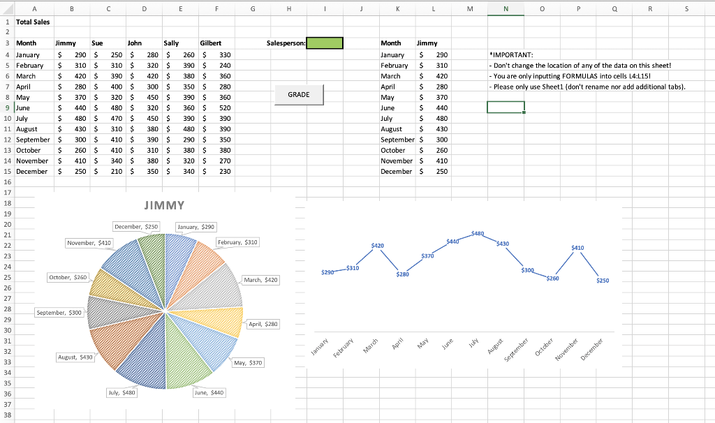
The “Assignment 5.2.xlsm” file contains monthly sales

Sometimes, you may not want to display all of your data. We're going to use a table of data containing five soccer players' names and their game rating for five games as we talk you through the process. Open the excel spreadsheet containing the data you want to chart. Click on the “insert” tab in the top toolbar. In this.

Range in Excel A Complete Guide to Working with Range and Cell

You can choose the methods which your think is perfect for you. Typically, you just need to highlight the cells containing the data. Create a chart by selecting cells from the table. We're going to use a table of data containing five soccer players' names and their game rating for five games as we talk you through the process. You.

Removing Cells From A Selected Range In Excel

With your data selected, navigate to the insert tab in the. Visualize your data with a column, bar, pie, line, or scatter chart (or graph) in office. Open the excel spreadsheet containing the data you want to chart. This article shows how to make dynamic charts in excel. In this post, you will learn two different methods to create a.

Create A Chart From The Selected Range Of Cells

You can choose the methods which your think is perfect for you. In this article, i will show you how you can create a chart from the selected range of cells. With your data selected, navigate to the insert tab in the. Once your data is ready, select the range of cells you want to include in your chart. Typically,.

Create A Chart From A Selected Range Of Cells - In insert, click recommended charts. Create a chart by selecting cells from the table. Typically, you just need to highlight the cells containing the data. Click on the “insert” tab in the top toolbar. With your data selected, navigate to the insert tab in the. In addition to creating dynamic chart ranges, i also show.

This article shows how to make dynamic charts in excel. Visualize your data with a column, bar, pie, line, or scatter chart (or graph) in office. Click on the “insert” tab in the top toolbar. Open the excel spreadsheet containing the data you want to chart. By following a few simple steps, you can easily select the right data and make an attractive, informative chart.

In This Post, You Will Learn Two Different Methods To Create A Dynamic Chart Range.

Sometimes, you may not want to display all of your data. Learn how to create a chart in excel and add a trendline. The first step is to create the. To create a chart, the first step is to select the data—across a set of cells.

Open The Excel Spreadsheet Containing The Data You Want To Chart.

Once your data is ready, select the range of cells you want to include in your chart. Visualize your data with a column, bar, pie, line, or scatter chart (or graph) in office. Create a chart by selecting cells from the table. Learn best ways to select a range of data to create a chart, and how that data needs to be arranged for specific charts.

Get The Sample File To Try The Methods.

To access the chart wizard, select the data range to be charted and press “f11”. In the insert chart window, go to all charts > column > clustered. The chart wizard is a guided feature within excel that helps users select data for their chart. In this article, i will show you how you can create a chart from the selected range of cells.

With Your Data Selected, Navigate To The Insert Tab In The.

Select the cells you want to include in your chart. We're going to use a table of data containing five soccer players' names and their game rating for five games as we talk you through the process. Click on the “insert” tab in the top toolbar. You can choose the methods which your think is perfect for you.